Small single-purpose models answer one question with one number between 0 and 1. What that number means, how to pick the cutoff, and how to check it against reality.

Bottom line. For any decision your system makes over and over, stop asking a large model to reason it out in a paragraph. Ask a small model to answer it with a number between 0 and 1, then pick a cutoff based on what each kind of error costs you in money. Check the number against a few hundred examples you labeled by hand. A raw score of 0.7 does not mean a 70 percent chance of anything until you have verified it. Watch precision at your actual cutoff rather than overall accuracy, which is close to meaningless when the thing you are looking for is rare. These models run on hardware you already own, add no per-call vendor charge, and nobody can deprecate them.
One question, one number
Most AI writing is about models that produce text. This is about the other kind.
A scorer takes some input and returns a single number between 0 and 1. That is the entire output. No paragraph, no explanation, no formatting to parse, no chance that it decides to be helpful and add a caveat you then have to strip out.
It means one thing, decided before you deployed it. Closer to 1 means this answer is supported by the source document. Or this message is toxic, this ticket is about billing, this tool call matches the request.
You set a cutoff. Above it, one thing happens. Below it, another. That is the whole design, and everything interesting is in where you put the cutoff and whether you trust the number.
Three you can try this week
Checking whether an answer is supported by its source. Vectara’s HHEM is built on DeBERTa-v3-base and takes two pieces of text, the source passage and the answer your system generated, then returns a factual consistency score. Zero means the answer has no support in the source. One means it is fully supported. Vectara suggests 0.5 as the cutoff. If you have a system that answers questions from your documents, this is a hallucination check with no API bill attached.
Checking whether text is toxic. CoreWeave’s toxicity scorer is a DeBERTa-v3-small with five separate heads for different categories of harm. It runs inside your own service in roughly 25 to 30 milliseconds per call on a CPU, with no external request and no data leaving your infrastructure.
Filtering before the expensive model runs. A common guardrail setup puts something small and fast in front, like ShieldGemma at 2 billion parameters or Qwen3-Guard at 600 million. Only the flagged portion goes to a larger model for a closer look.
At the far end of small, teams are training classifier heads of around sixteen thousand parameters that sit on top of embeddings they already compute. Not sixteen billion. Sixteen thousand. The decision costs microseconds of CPU time, no network call, and nothing leaves the machine.
Running one, step by step
I took a small open PII detector and ran it. The repository is a local binary classifier behind a Go HTTP gateway, with a Python service holding the model. It scores one piece of text and returns the probability that the text contains personal information.
Two commands get you to a dataset and a passing test suite.
python generate_synthetic_dataset.py --examples-per-category 200
go vet ./... && go test ./...
The Go tests passed in about three milliseconds per package and go vet was clean. Then I trained a scorer on the generated data and measured it. The author shipped fixes four times while I was writing, so I measured four times, and those measurements are the rest of this article.
The detector fine-tunes MiniLM-L12-H384-uncased, a 12-layer distilled transformer from Microsoft Research with a 384-dimensional hidden size. Small enough that the fine-tune runs on a MacBook Air in single-digit minutes, and the base weights download once.
One caveat about the measurements below. For the round-by-round comparisons I used a simpler stand-in scorer, a character-pattern model with 2,665 weights that trains in under a second, so I could re-measure after every change to the data. A fine-tuned transformer would transfer better than mine on the last test. The problems it exposed belong to the data rather than to either model.
Round one: a perfect score is a symptom
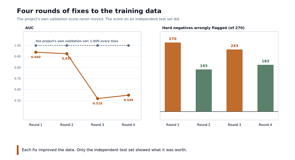
Against the project’s own validation file, my scorer returned an AUC of 1.000 with perfect precision and recall at every cutoff.
Perfect scores are a symptom rather than a success.
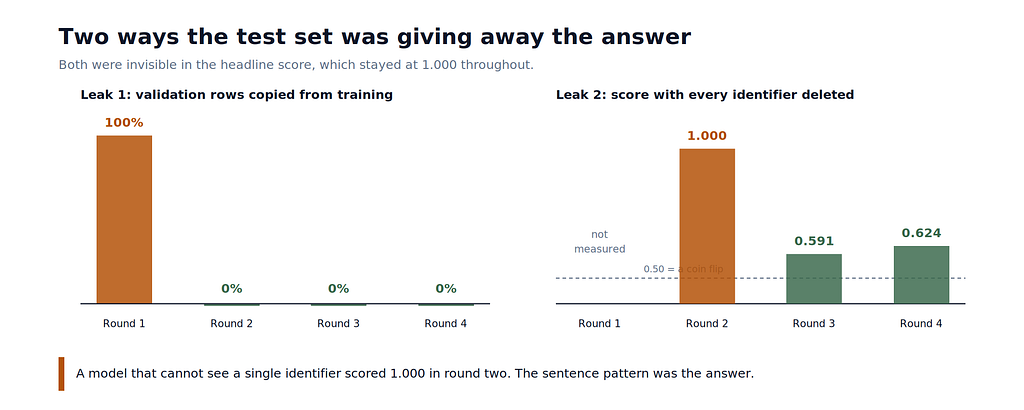
One query found the cause. The 880 validation rows contained only 102 unique sentences, and every one appeared word for word in the training file. The training file held 3,520 rows built from 113 unique sentences, each repeated about 31 times. The model had memorized a hundred sentences and been tested on the same hundred sentences.
I built my own test set. Same categories, entirely different values, plus hard negatives, meaning text that looks like personal information and is not. Order references. Invoice dates. A public support line. A build artifact whose name happens to be sixteen digits. A product SKU that reads like a national ID. 650 rows, 110 of them genuine, zero overlap with the training file.
AUC came back at 0.940, which sounds strong. Precision at the default 0.5 cutoff was 21.4 percent, so four of five flags were wrong, and all 270 hard negatives were flagged.
Round two: fixing the leak, and finding a subtler one
The author fixed it the same day. Values were now generated separately for each split, and the hard negatives I had been testing with were added to the training data.
Verbatim overlap went to zero. On my test set the hard-negative failures dropped from 270 of 270 to 165 of 270, and precision at the 0.9 cutoff rose from 42 to 59 percent.
The project’s own validation file still reported 100 percent.
This one was subtler than the first bug. Every sentence template belonged to exactly one label. “The account identifier is X” was always personal information and “Order reference X is ready to ship” was always safe, with no template appearing under both. A model could ignore the identifier entirely and classify on the sentence frame.
I tested that by deleting every identifier from every sentence, replacing all digits and emails with a placeholder, then training on the remaining frames. It scored AUC 1.000. A model that could not see a single identifier still graded perfectly.
The split name was also written into the data. Training addresses contained the literal word TRAIN and validation addresses contained VALIDATION, with email domains to match.
Round three: the independent number gets worse
The author fixed those too. Split markers gone, value formats shared across splits, and twelve sentence frames now used by both labels.
That template test confirms it. A model trained on sentences with every identifier deleted scored 0.591 instead of 1.000, barely better than a coin flip. The sentence frame no longer gives away the answer.
You can see the cause in the data. Round three generates values like contact8868036@example.test and 3524991 Example Avenue, Example City, EX 24991. My test set uses the kind of values a person would actually have, like kofi.mensah@sample.test and +65 6221 0000. The scorer learned those synthetic formats exactly, which is why it aces a test drawn from them and fails on anything else.
Round four: the trend turns
Round four added value variants, so emails and phone numbers appear in several formats rather than one, along with five more categories of safe text and an evaluation module that computes precision, recall, AUC, Brier score, and calibration error directly.
On my test set the hard-negative failures fell from 243 to 183 and AUC recovered from 0.518 to 0.549, the first improvement since round one.
At the 0.9 cutoff, the project’s own validation file finally showed a cost, with recall dropping to 83 percent and 373 cases missed. After three rounds of reporting a flawless score at every threshold, the file was measuring something real.
My character-pattern model is unusually sensitive to format, and a fine-tuned transformer would transfer more of the meaning across. Trust the direction here more than the exact numbers.
None of this is a criticism of the project, which documents these risks in its own dataset guide and shipped three rounds of fixes in a day. The rule it demonstrates is simple: synthetic data measures itself. A number produced on data you generated tells you about the generator, and only an independent test set tells you whether any of the work helped.
The cutoff is a business decision, not a technical one
Here are the measured rates from round one, where the detector was closest to usable.
At a cutoff of 0.5, the scorer catches 99.1 percent of the genuine cases and flags 74.1 percent of the clean ones. At 0.9, it catches 94.5 percent and flags 26.5 percent.
Two names to know. Every vendor uses them.
Recall is the share of real cases you caught. Precision is the share of your flags that were real. Raising the cutoff buys precision and sells recall, and no setting gives you both.
Now apply those measured rates to a realistic stream: 10,000 messages a day, 2 percent of which contain personal information. That is 200 genuine cases and 9,800 clean ones.
At the 0.5 cutoff, you catch 198 and miss 2, and you also flag about 7,259 clean messages. Somebody reviews 7,457 items to find 198 real ones. Precision 2.7 percent.
At the 0.9 cutoff, you catch 189 and miss 11, and flag about 2,595 clean ones. Somebody reviews 2,784 items. Precision 6.8 percent.
Doing the arithmetic in money
Price both kinds of error and the argument resolves itself.
Say a missed leak costs $500 in incident handling and notification. Say a review costs $2, a minute of somebody’s attention.
At 0.5: two misses at $500 is $1,000, plus 7,457 reviews at $2 is $14,914. Total about $15,900 a day.
At 0.9: eleven misses at $500 is $5,500, plus 2,784 reviews at $2 is $5,568. Total about $11,100 a day.
The higher cutoff wins. Now suppose reviews need a trained specialist at $25 rather than a minute of general attention.
At 0.5 the daily cost becomes about $187,400. At 0.9 it becomes about $75,100.
Same model, same scores, and the gap widens from under five thousand dollars a day to over a hundred thousand.
Now change the other number. Suppose a missed leak costs $5,000 rather than $500, which is not unusual once notification and regulatory exposure are involved, and reviews are back to $2.
At 0.5: two misses at $5,000 is $10,000, plus $14,914 in reviews. Total about $24,900.
At 0.9: eleven misses at $5,000 is $55,000, plus $5,568 in reviews. Total about $60,600.
The answer flips. The low cutoff now wins by thirty-five thousand dollars a day. Missing something became expensive enough to justify reviewing a lot of noise. For these measured rates, the crossover sits where a miss costs about 500 times a review.
The threshold question has no technical answer. Write down the two costs, multiply by the measured rates, compare.
It also shows when a model is not ready. Neither of those cutoffs is acceptable for production, and no threshold fixes a detector that flags every order number. The fix is training data containing order numbers labeled as safe.
The trap of rare events
The base rate moved between those two examples. On the test set, 17 percent of the rows contained personal information and precision was 21 percent. In the realistic stream at 2 percent, precision fell to 2.7 percent with the same model and the same cutoff.
Make it rarer still, one in a thousand, and precision collapses further. The model did not change. The world got rarer.
This arithmetic is one reason detection queues fill with false alarms, and it is worth checking before blaming the model. When the thing you are hunting is rare, even a good detector produces mostly false alarms. You fix it by raising the cutoff, by adding a second cheap check every flag must pass, or by accepting that the queue is mostly noise and staffing for it.
Why overall accuracy is a useless number
In the 2 percent stream, a model that says “no personal information here” every single time, flagging nothing at all, is right 98 percent of the time. At one in a thousand, that same do-nothing model is 99.9 percent accurate.
Accuracy rewards doing nothing whenever the interesting thing is uncommon. Ask for precision and recall at the cutoff you plan to use, and treat an accuracy figure on its own as a non-answer.
How to read AUC without being fooled
AUC has a plain meaning that rarely gets explained. Pick one text that contains personal information and one that does not, at random. AUC is the probability that the model scores the first one higher. 0.5 is a coin flip, 1.0 is perfect.
This detector scored 0.940, which sounds like a strong model, while delivering 21 percent precision at its default cutoff. AUC summarizes the model’s ranking without depending on where you set the cutoff, which is also its limitation. It tells you nothing about what happens at the cutoff you ship, and nothing about whether a score of 0.7 corresponds to anything.
Does 0.7 mean anything? The calibration question
When a scorer outputs 0.7, that does not mean there is a 70 percent chance the text contains personal information. It means the model’s arithmetic produced 0.7. Whether that matches reality is an open question until you check.
Checking takes an afternoon. Sort your labeled examples into buckets by score and compare the average score in each bucket to the share that turned out to be real.
That check on the detector, before any correction, looked like this.
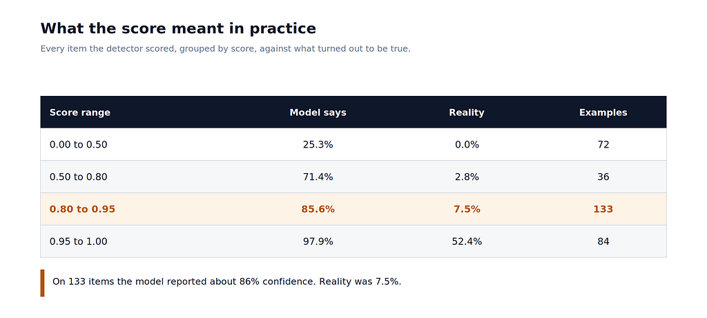
That average gap across all buckets has a name, expected calibration error. For this model it was 0.569. The Brier score, which is the average squared difference between the number and the outcome scored as 0 or 1, was 0.460. Both are bad.
Correcting a score that means nothing
The fix is old, cheap, and boring. Fit a small correction curve that maps raw scores onto accurate ones, using examples where you know the answer. The common method, Platt scaling, fits a simple S-shaped curve with two parameters. Isotonic regression learns a staircase instead and handles stranger distortions at the cost of needing more data.
I split the test set in half, fit the correction on one half, and measured on the other.
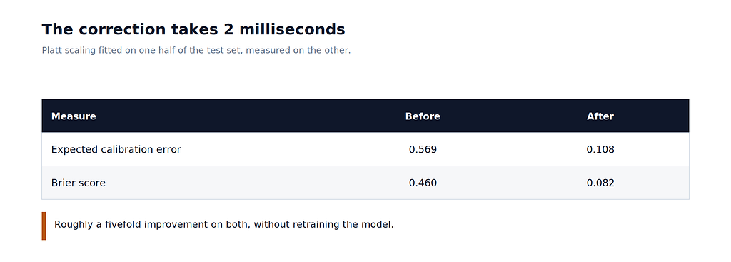
Calibration does not make the detector good. Precision stays poor while the training data stays wrong. Calibration buys a number that corresponds to a real rate, so you can set a threshold on purpose instead of by feel.
Do not ask the big model how sure it is
A tempting shortcut is to let a large model rate its own confidence and use that number.
Researchers tested this against an external scorer that checked claims against sources. The external scorer was better calibrated on every population they measured. Asking the model to state its confidence alongside its answer made it more confident, raising its average self-reported number, without making it any more accurate.
A model grading itself is performing a fluency task. A small scorer measured against labeled examples is taking a measurement.
How many examples do you need
Three hundred is usually enough, and most teams label far fewer.
How much a measured rate wobbles depends on how many examples you measured. Check 100 examples and find 70 percent precision, and the true figure sits around 70 give or take 9 points. At 300 examples that narrows to about 5 points. At 1,000, about 3 points.
Three hundred carefully labeled examples is a good default for a first pass, roughly a day of one person’s attention. My whole evaluation above used 650 rows, which took minutes to generate and would have taken a day to label by hand from real traffic.
What the whole exercise cost
My scorer trains in under a second and runs on a CPU. The Go gateway and the model service both bind to localhost, so no text leaves the machine. For a personal-information detector, that is the difference between a quick project and a compliance review.
That whole loop, generate data, train, score, calibrate, measure, ran on a MacBook Air in single-digit minutes. No GPU, no cluster, no vendor account, no API key.
Using synthetic data let me skip the slow parts. Labeling real examples takes about a day per three hundred. Agreeing on what counts as personal information takes a meeting, and usually more than one. Keeping both current as the traffic shifts takes somebody’s time every quarter. Budget for the model and not for those, and you pay for them later anyway.
Running the whole loop in minutes on a laptop let me measure four times in one afternoon. Every measurement said the same thing, which is that the detector was not ready.
Where this approach fails
Your inputs drift. A scorer calibrated on last quarter’s traffic can quietly go out of tune when the traffic changes. The number keeps arriving and keeps looking authoritative. Re-check it on fresh labeled data on a schedule.
The labels are the hard part. A scorer is only as good as the examples you were willing to label. Two people labeling the same items will disagree more than you expect. Have two people label the first fifty and compare before trusting anything downstream.
A number is not an explanation. When a human has to act on a borderline case, 0.62 tells them nothing. Show the score next to the input and let the person look.
Off-the-shelf does not mean off-the-shelf. A public scorer was trained on somebody else’s data, which rarely resembles yours. Measure it on your own labeled set before adopting it, and expect the published figures to be optimistic.
How to start
Pick one decision your system makes thousands of times. Routing, filtering, flagging, checking an answer against a source.
Write down in a single sentence what the number means. If you cannot, you have a definition problem rather than a modeling problem, and no model will solve it.
Label two or three hundred examples by hand.
Try an off-the-shelf model first, scored against your own labels. Train something only when the shelf comes up empty.
Build the cost table: what a false positive costs, what a false negative costs, and the volume of each at two or three candidate cutoffs. Pick the cutoff that minimizes the total.
Calibrate, then re-check the cutoff.
Then watch it. Score distribution, precision at the cutoff, and a monthly sample reviewed by a person.
The quieter half of the AI story
Most of the attention goes to models that write code and hold a conversation, and they have earned it. Meanwhile something less glamorous is happening inside production systems, where expensive general models are being replaced for specific repeated decisions by small ones that answer with a number.
These run on hardware you already own. They need no vendor relationship, and nobody retires them on a schedule you do not control. They answer one question, and you can prove whether they answer it correctly.
For a large share of what teams currently spend tokens on, that is a better deal.
Reader discussion