
The standup takes eleven minutes. Every item on the board is in progress, every update sounds the same. Almost done, just needs review. Almost done, just needs integration. Waiting on staging. Nobody is lying and nobody is slacking, and next week the same items give the same updates. The board is a wall of motion with no delivery coming out of it.
This piece is the second in a series on the small set of laws that govern how engineering organizations actually behave. The first covered Amdahl’s law and the serial fraction hiding in org charts. This one covers the two queueing results that explain the wall of 90 percent, plus the batch-size mistake that builds it.
Little’s Law: the arithmetic you can’t opt out of
In 1961 John Little published a proof of a relationship that operations people had assumed for years: the number of items in a system equals the arrival rate multiplied by the average time each item spends inside. Rearranged for our purposes, cycle time equals work in progress divided by throughput.
You already run this calculation in a supermarket line. Eight carts ahead, the cashier clears two carts a minute, four minutes until you check out. Little proved that the everyday version holds in general: for averages, over any window, in any system where work goes in one side and comes out the other.
The proof made Little famous because it needs almost nothing to be true. No assumptions about when items arrive, no assumptions about how long each one takes, no requirements on the order they’re processed. A hospital ward, a highway on-ramp, a Jira board. It does require the system to be roughly stable over the window you measure, meaning work enters at about the rate it leaves. A board where the count of open items grows every week has arrival outrunning throughput, and its average cycle time keeps climbing until one of the two changes.
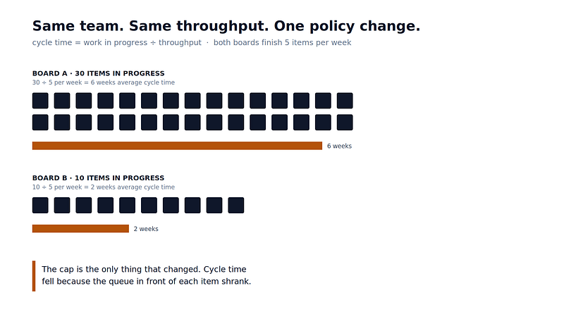
Run the numbers on the standup above. The team finishes five items in a typical week. The board holds thirty items in progress. Cycle time: thirty divided by five, six weeks. Average. Every item on that board will take a month and a half to cross it, and no amount of effort, urgency, or morning ceremony changes the result, because the result follows from the two inputs by arithmetic.
Most boards undercount their work in progress. The real count includes everything started and not yet delivered: the item in review, the item blocked on another team, the item waiting for a staging slot, the branch someone opened before vacation. The waiting states hold most of the calendar time, so leaving them out of the count understates the cycle time the team actually experiences.
Two levers exist. Raise throughput, which is slow and expensive, or lower work in progress, which is a policy decision available this afternoon. Cap the board at ten items and the same people, at the same throughput, post a two-week cycle time, because the queue in front of each item shrank. This is why WIP limits belong in the same category as gravity rather than in the category of team culture. A WIP limit sets the only free variable in an equation.
Kingman: the price of running full
Little’s Law says how long items take on average. Kingman’s formula, published the same year by John Kingman, says what happens to waiting as a system approaches full capacity, and the answer is the least intuitive result in this series. Wait time doesn’t grow linearly with utilization. It grows with utilization divided by idle capacity, multiplied by how variable the incoming work is.
Utilization is the fraction of time the team is busy; idle capacity is the rest. Dividing one by the other measures how much recovery room the system keeps. At 50 percent utilization, recovery room matches workload and the ratio is 1. At 95 percent, workload outweighs recovery room nineteen to one, and that ratio becomes the multiplier on your waiting.
Randomness arrives in clumps, and idle time is the only thing that absorbs a clump. A half-loaded team catches up during the quiet stretch after a burst. A team at 95 percent has almost no quiet stretches, so the delay from one burst is still unpaid when the next burst arrives, and delays stack instead of clearing. Waiting near full utilization compounds the way an unpaid balance does, because the schedule never contains a payment.
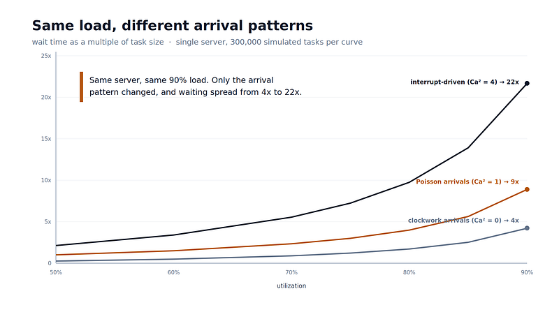
The natural model for incoming work is a Poisson process: tickets, pages, and requests arriving independently at a steady average rate, with no memory, meaning the time since the last ticket tells you nothing about when the next one comes. Poisson arrivals describe most real intake streams well, which is why the model has run call centers and telephone networks for a century. I simulated 300,000 tasks flowing through a single server under Poisson arrivals, sweeping the load upward. At 50 percent utilization, a task waits about as long as its own size. At 80 percent, four times its size. At 90 percent, nine times.
Then I changed only the arrival pattern and ran it again, twice. Arrival variability has a score, Ca², which measures how clumped the gaps between arrivals are: zero for a metronome, one for Poisson, higher as work bunches. With clockwork arrivals at Ca² of zero, the same rate landing at perfectly even intervals, the wait at 90 percent load dropped to four times task size. With bursty arrivals at Ca² of four, which is what an interrupt-driven intake looks like, the wait hit twenty-two times task size. Same server. Same average load. The spread between the calmest and spikiest pattern was more than a factor of five, and every bit of it came from variability. The full simulation runs about fifty lines of Python; here is the notebook code, including the comparison against Kingman’s formula and the chart below.
import math
import random
N_TASKS = 300_000 # tasks per run
WARMUP = 30_000 # discarded so steady state dominates
UTILS = [0.50, 0.60, 0.70, 0.75, 0.80, 0.85, 0.90]
def make_sampler(kind, mean_inter, rng):
"""Return a function that samples one gap between arrivals."""
if kind == "clockwork": # Ca^2 = 0: even intervals
return lambda: mean_inter
if kind == "poisson": # Ca^2 = 1: independent arrivals
return lambda: rng.expovariate(1.0 / mean_inter)
if kind == "bursty": # Ca^2 = 4: clumped arrivals
c2 = 4.0 # two exponential branches, one
p1 = 0.5 * (1 + math.sqrt((c2 - 1) / (c2 + 1))) # fast and
r1 = 2 * p1 / mean_inter # frequent,
r2 = 2 * (1 - p1) / mean_inter # one slow
return lambda: (rng.expovariate(r1) if rng.random() < p1
else rng.expovariate(r2))
def simulate(util, kind):
"""Mean wait, in multiples of mean task size, at this load."""
rng = random.Random(42)
sample_gap = make_sampler(kind, mean_inter=1.0 / util, rng=rng)
t = server_free = total_wait = 0.0
for i in range(N_TASKS):
t += sample_gap() # next task arrives
start = max(t, server_free) # waits if server is busy
server_free = start + rng.expovariate(1.0) # service, mean 1
if i >= WARMUP:
total_wait += start - t
return total_wait / (N_TASKS - WARMUP)
for kind, ca2 in [("clockwork", 0.0), ("poisson", 1.0), ("bursty", 4.0)]:
for u in UTILS:
kingman = u / (1 - u) * (ca2 + 1) / 2
print(f"{kind:>9} {u:.0%} sim {simulate(u, kind):6.2f}x"
f" kingman {kingman:6.2f}x")
Now look at how teams get planned. Capacity spreadsheets allocate every engineer to 100 percent. A team with visible slack reads as underutilized, and underutilized reads as a problem to fix. The spreadsheet is optimizing exactly the number Kingman says to fear, and it is blind to the variability term entirely. A team loaded past 90 percent runs as a queue in which everything waits many times longer than the work itself takes, and each new “small ask” joins the back of that queue.
The two knobs in the simulation map directly onto kinds of teams. Planned feature work approximates clockwork: arrivals are scheduled, smooth, and forgiving, so a feature team can run hot. Incidents, escalations, and questions approximate the bursty curve, so a team fielding them at 90 percent load lives at the top of the chart, waiting twenty-two tasks deep. Those interrupt-driven teams need the most slack and usually get the least, because their work is the hardest to see on a roadmap and their idle time is the easiest to spot on a spreadsheet. Utilization measures cost while flow measures output, and past 80 percent the two move in opposite directions.
Batch size: why the last 10 percent is half the work
The third mechanism is the one that manufactures 90-percent-done items specifically. A batch is the amount of work that travels together: the size of the pull request, the scope of the release, the number of changes deploying at once. Donald Reinertsen spent a career documenting what batch size does to product development, and the summary is that large batches delay feedback, hide defects, and concentrate risk at the end, which is exactly where the standup finds it.
A large change sits at 90 percent because the remaining 10 percent is where the batch meets reality: integration, review, deployment, the collision with everyone else’s large change. The first 90 percent was typing, and the batch deferred every piece of feedback into the last 10. Meanwhile a large change is slow to review, so it queues longer per Kingman. It occupies work in progress the whole time, so it inflates cycle time per Little. And when a defect surfaces in a 3,000-line change, the search space is 3,000 lines; in a 200-line change, the search is an afternoon.
Large batches have a rational origin. Every release carries a fixed overhead: the deploy checklist, the regression pass, the approval form. When the overhead per release is high, packing more work into each one looks efficient, and by the local math it is. So the lever is the cost of a release rather than anyone’s discipline. Automate the deploy, shrink the checklist, make shipping cheap, and small batches stop costing anything. Teams batch big when each release is expensive, and they stop on their own when it’s cheap.
Batch size also feeds the Kingman machine from the service side. A mix of one-day changes and three-week changes has the same spiky profile that multiplied the waiting in the simulation, applied to task sizes instead of arrival times. Uniformly small changes calm both terms at once. A change that takes a day to build and an hour to review moves through every queue faster, fails cheaper, and finishes instead of progressing. An item that has been 90 percent done for two weeks was scoped wrong two weeks ago, and its status reports the batch size, not the work.
What to change on Monday
Compute your real numbers first. Count everything started and undelivered, including items in review and items blocked, count items finished per week, divide. If the cycle time that falls out surprises you, that surprise is the whole argument.
Then cap work in progress below where it sits today. One to two items per person is the usual starting point, and the exact number matters less than holding it when it becomes annoying, because it becomes annoying precisely when it starts working: the moment someone wants to start a new item and can’t, the system is forcing a finish instead. Watch item age as the leading indicator, since cycle time only confirms problems after they’ve finished; anything older than twice your target gets swarmed or split.
Split anything expected to run past a few days of work into changes that can each ship, and spend real engineering time making a release cheap, since release overhead is what makes big batches look sensible. And leave deliberate slack in the plan for any team with interrupt-driven arrivals, over the objection of the utilization spreadsheet, which is measuring cost while you are trying to buy flow.
None of this requires a transformation, a framework, or a consultant. Little’s Law is division and Kingman is a curve. The board full of 90-percent-done items is what those two results look like from inside, and both of them respond to policy within a week.
By Joshua McDonald on July 27, 2026.
Reader discussion